Create Pivot Table From Multiple Worksheets Excel 2016 Mac

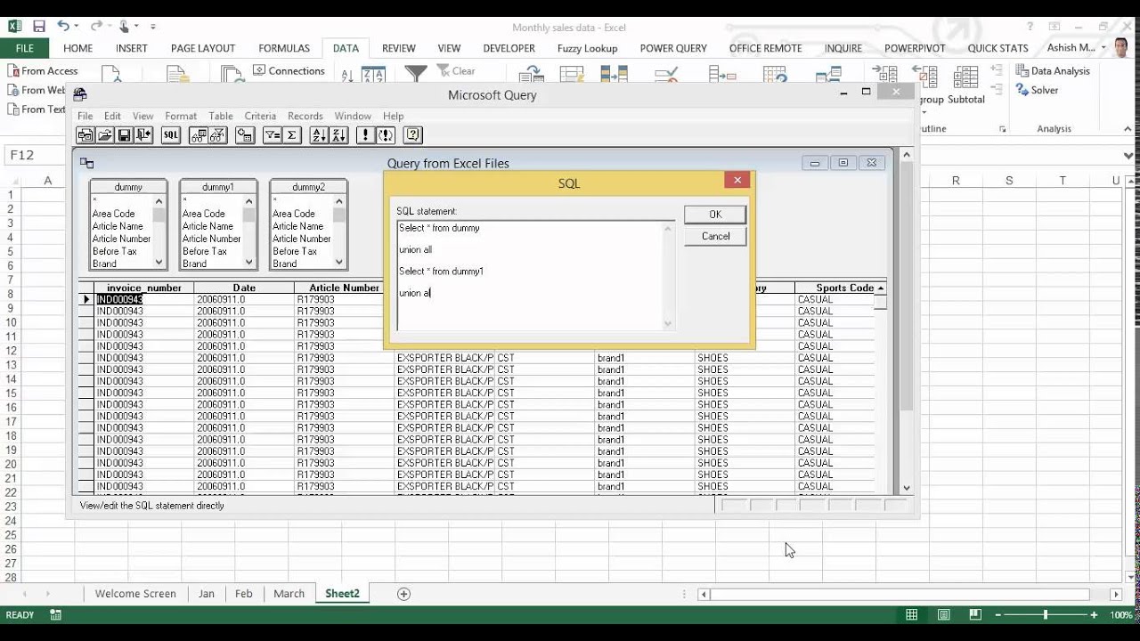
From the File Menu - click on Return Data to Microsoft Excel. Here we will use multiple consolidation ranges as the source of our Pivot Table.
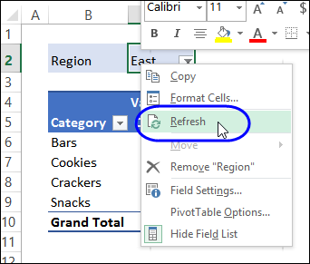
Automatically Refresh An Excel Pivot Table Excel Pivot Tables
The steps below will walk through the process of creating a Pivot Table from Multiple Workbooks.

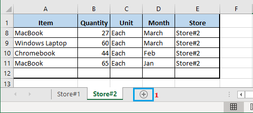
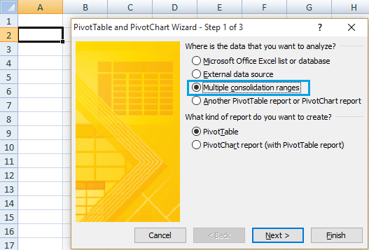
Create pivot table from multiple worksheets excel 2016 mac. Click the button to open the PivotTable and PivotChart Wizard. Also if you add more data to any of the 4 sheets the pivot table will update as soon as you refresh it. It will create multiple worksheets in the same file.
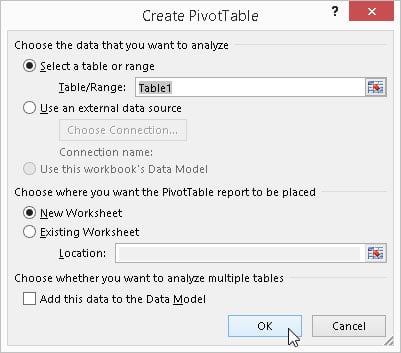
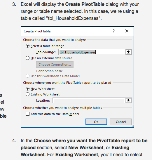
In the Create PivotTable dialog box under Choose the data that you want to analyze click Use an external data source. Creating a Pivot Table with Multiple Sheets. In this window go to the Data tab.
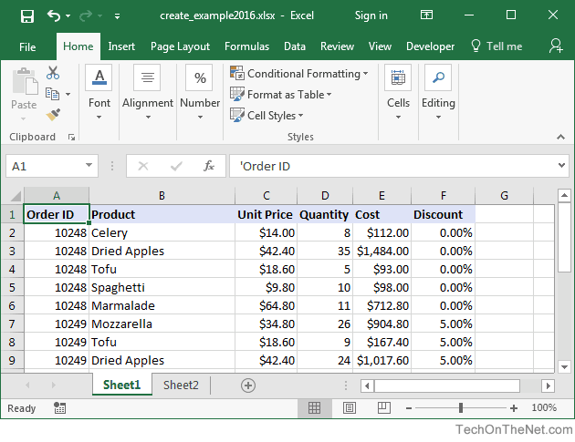
Excel will ask you to verify that your data has a header row. Each month is on a different tab and the tables are set up so that each row is an employee and each column is a different cost center that their time gets charged to. We can use the Power Table Wizard in Excel to create a pivot table from multiple worksheets.
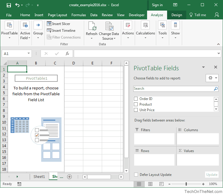
The following dialogue box will appear. Click a blank cell that is not part of a PivotTable in the workbook. Click Insert PivotTable.
On Step 1 page of the wizard click Multiple consolidation ranges and then click Next. Select ALTD then P and the PivotTablePivotChart Wizard will open. In that dialogue box select Multiple consolidation ranges and click.
Under Choose commands from select All Commands. Select either PivotTable or PivotChart report. Easy is a relative concept.
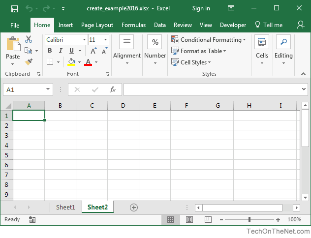
Click any cell on the worksheet. Create Second Pivot Table in Same Worksheet Now you can create a second Pivot Table in the same Worksheet by following the steps below. Select to create the Pivot table in a new Worksheet and click on Finish.
Select Multiple consolidation ranges. To activate this click on Options in the File Tab and click on Customize Ribbon select All Commands in the Choose commands from field and scroll till you find PivotTable and PivotChart. In the Data Tab Uncheck Save Source Data with File.
Alt D is the access key for MS Excel and after that by pressing P after that well enter to the Pivot table and Pivot Chart Wizard. Figure 1- How to Create a Pivot Table from Multiple Workbooks. On the Tables tab in This Workbook Data Model select Tables in Workbook Data Model.
In the list select PivotTable and PivotChart Wizard click Add and then click OK. Select the range on the first worksheet. In the end import the data back to excel as a pivot table.
Yes it is easy once you know how to do it. Label the Page field appropriately. In the wizard select Multiple consolidation ranges option and the PivotTable option and then click the Next button.
How to Create a Pivot Table from Multiple Worksheets. We must put the data in a table form. Below are the steps to create pivot table from multiple sheets Click AltD then click P.
By default these three tables will be called Table1 Table2 and Table3. In Excel for Mac you can use Microsoft Query to make a PivotTable using multiple worksheets from an Excel workbook as your data source. Now proceed with Show Filter Report Pages.
Go to each worksheet and MoveCopy it to a new file and save it. An instructional video on how to create a Pivot Table in Microsoft Excel 2016 on a Mac. Create a Pivot Table From Multiple Tables - YouTube.
Click OK to create the table. If you wish to create the pivot table in same sheet input the desired cell information from where the. Add the worksheet ranges for the table.
On each of the three worksheets select the individual data set and press CtrlT. Setting up the Data. After doing this Save the file again.
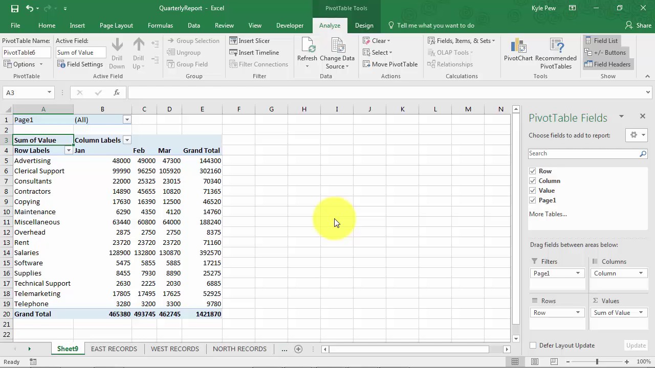
The steps below will walk through the process of creating a Pivot Table from Multiple Worksheets. Excel for Mac 2016 - Pivot Table data from multiple tabs in workbook I have workbook for our employee time allocations. Select Create a single page field for me.
Select data from both the sheets and create one Page Field for each sheet. Open the file in Excel 2016. Setting up the Data.
Click on any empty cell in the same Worksheet Make sure the Cell is away from the first pivot table that you just created. We will click on any cell in the table click on the Insert tab click on. You can see that in total from all 4 sheets we have 592 records.
We will open a New excel sheet and insert our data. In a case where the data you want to summarize in this Pivot Table are in say 3 worksheets in the same workbook a simple method will be to make use of the PivotTable and PivotChart Wizard.
How To Create Pivot Table From Multiple Worksheets

Pivot Table Tips Exceljet
Ms Excel 2011 For Mac How To Create A Pivot Table
Create An Excel Pivottable Based On Multiple Worksheets Youtube
How To Create Pivot Charts In Excel 2016 Dummies
Ms Excel 2016 How To Create A Pivot Table

Pivot Table Tips Exceljet

Pivot Table Tips Exceljet
Microsoft Excel For Mac Pivot Tables Microsoft Community

How To Create A Pivot Table From Multiple Worksheets Step By Step Guide
Create A Pivot Table From Multiple Worksheets Of A Workbook Youtube
Ms Excel 2016 How To Create A Pivot Table
How To Create Pivot Table From Multiple Worksheets
Pivot Tables Including Data From Multiple Sheets Microsoft Community
Ms Excel 2013 How To Create A Pivot Table
Pivotpal A Fast New Way To Work With Pivot Tables Excel Campus
How To Create Pivot Table From Multiple Worksheets

How To Create A Pivot Table In Excel To Slice And Dice Your Data Digital Trends
Ms Excel 2016 How To Create A Pivot Table